Short Description of the Project
In classical Traveling Salesman Problem (TSP), a virtual salesman must have to find the most efficient sequence of some given cities. But, the conditions are, the salesman must visit all the given cities, the salesman can visit a city only once and the salesman must return back to the starting city. Genetic algorithm (GA) is one of the well-known and most frequently used algorithm for solving TSP. If the operators of GA can be designed properly, it can provide optimal/near-optimal solution within a very short time. In this project, we implemented several mutation operators in classical GA. We designed a mutation triggering method by combining three mutation operators (Swap, Insertion and 2-Opt) and applying adaptive probability. To decide which mutation will be activated at a given generation, a decision-making method named Mutation Triggering Method is proposed.
Tools and Technologies Used
- Programming Language: Java
- Machine: Intel(R) Core(TM) i5-2430M machine with 2.40 GHz processor and 8.00 GB RAM
- Operating System: Windows 10 (64 bit)
- IDE: Eclipse 4.7 (Oxygen)
- JDK: 8
Dataset
- TSPLIB instances (eil51, a280, bier127, kroa100, kroa200, lin318, pr226, st70, rat195)
Implemented Algorithms
- Traditional Genetic Algorithm (T-GA)
- Random Crossover and Dynamic Mutation Genetic Algorithm (RCDM-GA)
- Mutation Triggering Method Genetic Algorithm (MTM-GA)
Implemented Strategies for Genetic Algorithms
- Population: Random population generation method
- Fitness function: f = 1/D; where, D = total travel distance of a tour = d1 + d2 + …… + dn and dn = Euclidian distance between two connected cities
- Selection: Tournament selection
- Crossover: Order crossover
- Mutation:
- 2-opt mutation
- Swap mutation
- Insertion mutation
Flowchart of the Algorithm
We followed the basic structure of the genetic algorithm except for the mutation operator phase. The improved algorithm is shown in Figure 1. The steps of the algorithms are described below:
Generate Initial Random Population: In this step, a fixed number of initial population was generated without any heuristic. We choose random population generation method.
Calculate Fitness of the Individuals: This step calculated the quality of each individual through a fitness function. To solve TSP, the fitness value of each chromosome is calculated by the equation, f = 1/D; where, D = total travel distance of a tour = d1 + d2 + …… + dn and dn = Euclidian distance between two connected cities ci and ci+1.
Stopping Criterion: This step is the stopping criterion of the algorithm. The algorithm runs for a fixed number of generations (by checking the condition, Generation < Max Generation) without considering the fact that it finds a better solution or not.

Crossover Operator: Apply Order Crossover on two Selected Individuals. In this part, if the crossover probability allows the operation, two selected individuals perform recombination by following the Order Crossover strategy.
Calculate Probability, pm According to the Progression of the Generation: This step is one of the most crucial parts of the algorithm since the mutation probability Pm is calculated here. The Mutation is a very sensitive operator that cannot be changed drastically. A higher probability of mutation might end up the algorithm to divergence with large computation time. On the other hand, a very smaller mutation probability might cause local optima. That is why, the mutation probability is reduced smoothly with the succession of the generation by following the equation, Pm = k / √(Current generation number); Here, k is a constant factor chosen over a range of [0, 1].
Mutation Selector Method: This step decides which mutation should be selected from 2-opt, Swap and Insertion mutation according to a selector equation. The 2-opt mutation is very effective to find cycles in the tour but the major drawback is that it is very slow. Applying 2-opt alone might cause greater computation time. On the other hand, Swap and Insertion mutations are very faster approach but provide low-quality solutions. Therefore, in this work, these three mutation methods are combined to ensure diversity as well as lesser computation time. A selector variable is defined that decides when to choose 2-opt mutation according to the factor constant, shown in the following equation, selector= max. generation − (factor ∗ max.generation)
For example, if the factor value is set as 0.2, it means that 2-opt will be triggered on the last 20% of the generations to generate a high-quality solution, sacrificing the higher computation time. On the other hand, the beginning 80% of the generation will take the benefits (faster) of Swap and Insertion mutations. Between Swap and Insertion mutation, a fair coin toss is performed.
Implementing the Mutation Triggering Method (MTM)
To be specific, designing MTM is the main objective of this project. This function decides which mutation operator will be selected according to some ideas. The algorithm of MTM is shown in Algorithm 1, below.

Experimental Result Based on Travel Cost

Experimental Result Based on Computation Time

Convergence Analysis
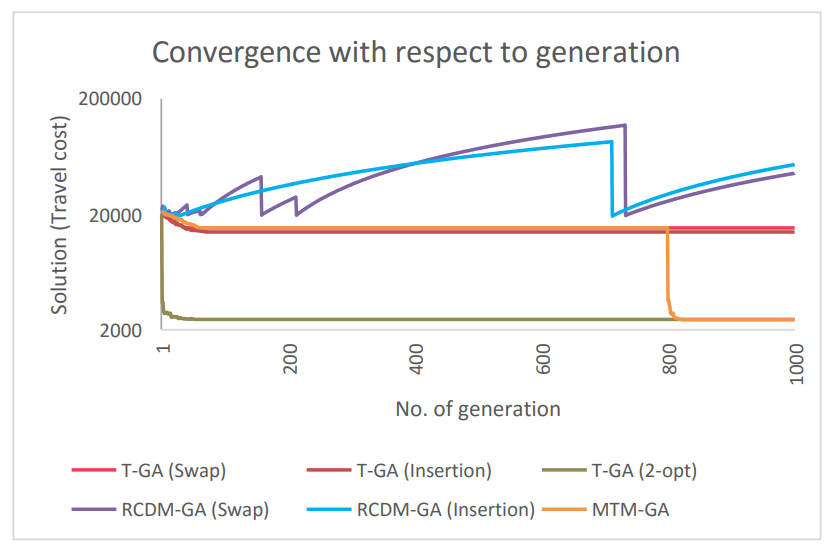
We considered one instance rat195 to experiment how all of the algorithms converge with the progression of the generation. After 1000 generation the solution for each generation was shown in Figure 1. It can be concluded that because of being random in nature, T-GA (Swap) and T-GA (Insertion) quickly get stuck in local optima, implies that unable to bring diversity. Since T-GA (2-opt) is a heuristic approach, it finds the optimal/ near-optimal solution within the first few generations. Running the algorithm for a long generation does not bring much diversity in this case. On the other hand, RCDM- GA (Swap) and RCDM-GA (Insertion) is too much random in nature. Since the mutation probability calculating function of RCDM-GA increases the probability when the solution does not vary, it fluctuates the solution for large dataset instances. It is generally effective for small dataset instances. However, MTM-GA is designed in such a way that it can use the benefits of both randomness and knowledge-based mutation operations. It quickly converges to the local optima using the random mutations. To escape from local optima, it uses heuristic mutation such as 2-opt mutation. The major improvement of TMT-GA is that it concentrates not only on optimality but also in computation time.