In this project, we implemented several heuristics to assess their effects in mobile robot path planning in uncertain and dynamic environment. Our goal is to find a path for the robot that is optimal, considering the simulation time and travel-distance. In order to analyze the robustness of our proposed heuristics, we plugged each of these heuristics in several search algorithms.
Machine: Intel(R) Core(TM) i5-2430M machine with 2.40 GHz processor and 8.00 GB RAM
Operating System: Ubuntu 14.04 LTS (32 bit)
IDE: Eclipse CDT 3.8
Implemented Algorithms
Dijkstra’s Algorithm
Greedy Breadth-first Search (GBFS) Algorithm
A* Algorithm
Optimized Cost Function A* (OCF A*) Algorithm
System Architecture
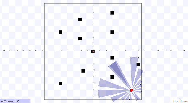
In our project, we designed the environment first that includes static and dynamic obstacles. An example of our environment and robot navigation is shown in Figure 1. The black objects are static obstacle that does not move with respect to time. The orange objects are dynamic obstacles that move with respect to time, and the velocity and position of these obstacles are uncertain. The red object is the robot. We choose Pioneer 3-DX robot for this project. In figure 2, we illustrated the system architecture. The robot sense the environment with IR sensor. The robot is controlled by two units. One unit does dynamic path planning that helps the robot to avoid the unknown obstacles. On the other hand, another unit does the global path planning that already knows about the position of the static obstacles. Based on the planning, the robot navigates from one point to another point (goal).
Figure 1: An uncertain and dynamic environment
Figure 2: The system architecture of our project
Implemented Heuristics
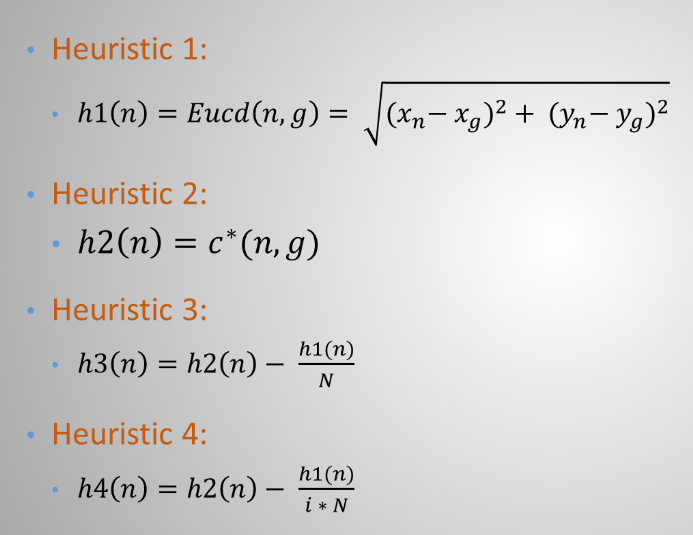
We implemented four heuristics in GBFS, A* and OCF A* algorithms. The heuristics are shown in Figure 3. Heuristic h1 is a Euclidean distance of the start and goal. But, it considers the static obstacles. Heuristic h2 is a true straight line distance that does not consider and obstacle. h3 and h4 are meta-heuristics, combining h1 and h2. Heuristic h3 also considers the total no of states N. Heuristic h4 considers N and introduce a new variable i, presenting the i-th iteration of the loop. It gives a feedback to the algorithm about the current generation. We plugged these four algorithms to each of the three heuristic algorithms GBFS, A* and OCF A*.
Figure 3: Four heuristics for GBFS and A*
Proposed Dynamic Planning Algorithm and A Sample Run for Each Algorithms
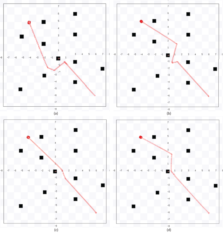
Figure 4 shows the flowchart of the Dynamic Planning Algorithm and figure 5 shows the sample of simulated path for four algorithms.
Figure 4: Flowchart of the Dynamic Planning algorithm
Figure 5: A Sample of simulated paths for static environement ; (a) Dijkstra’s (b) Greedy BFS (c) A* (d) OCF version of A*
Experimental Results
Comparison Criterion:
Comparison with static obstacle
Comparison with uncertain and dynamic obstacles: a) Keeping initial positions of the obstacles fixed b) Keeping initial positions of the obstacles random
Performance Metrics:
Simulation Time
Travel-distance
Comparison for static obstacles:
Figure 6: Simulation time (static obstacles)
Figure 7: Travel-distance (static obstacles)
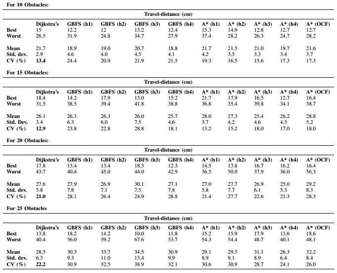
Comparison for uncertain and dynamic obstacles with fixed initial positions (for 10, 15, 20, and 25 obstacles):
Figure 8: Simulation time (uncertain & dynamic obstacles with fixed initial position)