Short Description of the Project
Using information from the World Happiness Report, this project investigates the ways in which economic, social, and governance issues affect national happiness. Multiple linear regression analysis was used to determine the influence of important variables on happiness scores across nations, including GDP, social support, healthy life expectancy, freedom to make life choices, generosity, and perception of corruption. To find out if high-income countries are significantly happier than low-income ones, countries were also categorized by income level for hypothesis testing.
According to the regression model, GDP, health, social support, freedom, generosity, and corruption were all significant predictors. With a low p-value, a hypothesis test employing the permutation method verified a statistically significant difference between high and low- income groups.
The results imply that national circumstances and socioeconomic status both have a significant impact on happiness. Policymakers and development projects aimed at enhancing general well-being through financial and social investments can be guided by these ideas.
Tools and Technologies Used
- Programming Language: R
- Machine: Intel(R) Core (TM) i7-6700Q CPU with 2.60 GHz processor and 16.00 GB RAM
- Operating System: Windows 10 (64 bit)
- IDE: RStudio
Data Collectiom
- Gallup World Poll surveys are used to gather the data for the World Happiness Report, a project of the Sustainable Development Solutions Network (SDSN)
- Data is compiled from a variety of sources, such as economic data, government documents, and polls that rely on perceptions
- The data source is available at: https://worldhappiness.report/data-sharing/
Independent Variables
- Country name: List of the country involved
- Year: Year the data was conducted
- Rank: A country’s position in the global happiness list based on its average life evaluation (Life Ladder) score for a given year
- Log GDP per capita: Gross Domestic Product, or how much each country produces, divided by the number of people in the country. Information about the strength of a nation’s economy
- Social support: Dependency on someone in times of trouble
- Healthy life expectancy: Number of years an individual is expected to live in good health which combines both the length of life and the quality of life.
- Freedom to make life choices: Right to life and liberty, freedom from slavery and torture, freedom of opinion and expression, the right to work and education
- Generosity: Charity, donation and community engagement
- Perception of corruption: The perception of government corruption, business corruption and individual corruption
Dependent Variable
- Ladder score (Happiness Score): An individual’s self-assessed rating of their current life on a scale from 0 (worst possible life) to 10 (best possible life), based on the Cantril ladder
Research Question
- How do economic, social, and governance factors influence national happiness scores across countries?
- Is there a significant difference in happiness scores between high-income and low-income countries?
Add Libraries and Load Data
library(tidyverse)
library(readxl)
library(GGally)
library(corrplot)
library(broom)
library(patchwork)
library(glmnet)
library(ggplot2)
library(infer)

happiness_data <- read_excel("/World_happiness_data_region.xlsx")

str(happiness_data)
## tibble [1,969 × 14] (S3: tbl_df/tbl/data.frame)
## $ Year : num [1:1969] 2024 2023 2022 2021 2020 ...
## $ Rank : num [1:1969] 1 143 137 146 150 153 154 145 141 154 ...
## $ Country name : chr [1:1969] "Finland" "Afghanistan" "Afghanistan" "Afghanistan" ...
## $ Ladder score : num [1:1969] 7.74 1.72 1.86 2.4 2.52 ...
## $ upperwhisker : num [1:1969] 7.81 1.77 1.92 2.47 2.6 ...
## $ lowerwhisker : num [1:1969] 7.66 1.67 1.79 2.34 2.45 ...
## $ Explained by: Log GDP per capita : num [1:1969] 1.749 0.628 0.645 0.758 0.37 ...
## $ Explained by: Social support : num [1:1969] 1.78 0 0 0 0 ...
## $ Explained by: Healthy life expectancy : num [1:1969] 0.824 0.242 0.087 0.289 0.126 ...
## $ Explained by: Freedom to make life choices: num [1:1969] 0.986 0 0 0 0 0 NA NA NA NA ...
## $ Explained by: Generosity : num [1:1969] 0.11 0.091 0.093 0.089 0.122 ...
## $ Explained by: Perceptions of corruption : num [1:1969] 0.502 0.088 0.059 0.005 0.01 ...
## $ Dystopia + residual : num [1:1969] 1.782 0.672 0.976 1.263 1.895 ...
## $ Region : chr [1:1969] "Western Europe" "Asia-Pacific" "Asia-Pacific" "Asia-Pacific" ...Rename the Columns
The column names of the original dataset is too large that might obscure the essential information in the plots. Therefore, the column names are renamed with shorter names as below:
happiness_data <- happiness_data %>%
  rename(
    Year = Year,
    Rank = Rank,
    Country = `Country name`,
    Score = `Ladder score`,
    UpperWhisker = upperwhisker,
    LowerWhisker = lowerwhisker,
    GDP = `Explained by: Log GDP per capita`,
    SocialSupport = `Explained by: Social support`,
    Health = `Explained by: Healthy life expectancy`,
    Freedom = `Explained by: Freedom to make life choices`,
    Generosity = `Explained by: Generosity`,
    Corruption = `Explained by: Perceptions of corruption`,
    DystopiaResidual = `Dystopia + residual`,
    Region = `Region`
  )

colnames(happiness_data)
## [1] "Year" "Rank" "Country" "Score"
## [5] "UpperWhisker" "LowerWhisker" "GDP" "SocialSupport"
## [9] "Health" "Freedom" "Generosity" "Corruption"
## [13] "DystopiaResidual" "Region"Discard Missing Values and Create Dataset with All Variables
The following dataset considers all the variables regardless of numerical and categorical variables. Also, for this project we discarded the missing values:
happiness_allVar <- happiness_data %>%
  select(
    GDP,
    SocialSupport,
    Health,
    Freedom,
    Generosity,
    Corruption,
    Rank,
    Score,
    Year,
    Rank,
    Country,
    UpperWhisker,
    LowerWhisker,
    DystopiaResidual,
    Region
  ) %>%
  na.omit()
Research Question 1: How do economic, social, and governance factors influence national happiness scores across countries?
To answer this question, we separated the numerical and categorical variables into different dataframes. For each numerical variables a linear regression model is designed to see how that variable can explain the target variable- happiness score. In the end, a multiple linear regression model is designed to see what are the significant factors that impact the happiness score. We added categorical variables to the multiple linear regression as well to see if the model accuracy increases.
Correlation Matrix (Numerical Variables) and Distribution
happiness_subset <- happiness_data %>%
  select(
    GDP,
    SocialSupport,
    Health,
    Freedom,
    Generosity,
    Corruption,
    Rank,
    Score,
  ) %>%
  na.omit()

ggpairs(happiness_subset)
From the ggpairs plot, we can see that Rank is highly correlated to Score (-0.98), therefore discarded from the analysis. Rank is the inverse representation of Score. A country with higher Score should have lower Rank. Other explanatory variables such as GDP, Social Support, Health, Freedom, Corruption has higher correlation with Score. Therefore, these variables could be useful to explain Score of a country. On the other hand, Generosity has the lowest correlation (0.043) with Score. This variable can be useful to improve the model accuracy.
Analysis of GDP versus Score
To find how GDP is related to Score, a linear model can be used as below:
lm_gdp <- lm(Score ~ GDP, data = happiness_subset)
happiness_augmented <- augment(lm_gdp)

summary(lm_gdp)
##
## Call:
## lm(formula = Score ~ GDP, data = happiness_subset)
##
## Residuals:
## Min 1Q Median 3Q Max
## -3.4711 -0.4444 0.0054 0.5490 2.1836
##
## Coefficients:
## Estimate Std. Error t value Pr(>|t|)
## (Intercept) 3.49940 0.07793 44.90 <2e-16 ***
## GDP 1.66807 0.05969 27.95 <2e-16 ***
## ---
## Signif. codes: 0 '***' 0.001 '**' 0.01 '*' 0.05 '.' 0.1 ' ' 1
##
## Residual standard error: 0.8158 on 866 degrees of freedom
## Multiple R-squared: 0.4742, Adjusted R-squared: 0.4736
## F-statistic: 781.1 on 1 and 866 DF, p-value: < 2.2e-16From the model equation and summary it can be said that for one unit increase in GDP, Score increases by 1.66807. The p-value (2e-16) is much lower than alpha = 0.05, indicating GDP to be a significant predictor for Score. The R-square value reveals that around 47.42% of Score can be interpreted by GDP.
A linear regression line and model diagnosis plots are presented below for validation. The residual plot shows that the model preserves linearity since the fitted values are evenly scattered on both sides of horizontal axis, and shows no pattern. The histogram and Q-Q plot also confirms the normality condition. Since the residual plot does not show any cone or funnel shapes, variability condition is also met.
# Create each plot
p1 <- ggplot(data = happiness_subset, aes(x = GDP, y = Score)) +
  geom_jitter() +
  geom_smooth(method = "lm") +
  ggtitle("GDP vs Happiness Score") +
  theme_minimal()

p2 <- ggplot(data = happiness_augmented, aes(x = .fitted, y = .resid)) +
  geom_point() +
  geom_hline(yintercept = 0, linetype = "dashed") +
  xlab("Fitted values") +
  ylab("Residuals") +
  ggtitle("Residuals vs Fitted") +
  theme_minimal()

p3 <- ggplot(data = happiness_augmented, aes(x = .resid)) +
  geom_histogram(bins = 25, fill = "steelblue", color = "black") +
  xlab("Residuals") +
  ggtitle("Histogram of Residuals") +
  theme_minimal()

p4 <- ggplot(data = happiness_augmented, aes(sample = .resid)) +
  stat_qq() +
  stat_qq_line() +
  ggtitle("QQ Plot of Residuals") +
  theme_minimal()

# Combine the four plots into a 2x2 grid
(p1 | p2) / (p3 | p4)
Analysis of Social Support versus Score
To find how Social Support is related to Score, a linear model can be used as below:
lm_socialsupport <- lm(Score ~ SocialSupport, data = happiness_subset)
happiness_ss_augmented <- augment(lm_socialsupport)

summary(lm_socialsupport)
##
## Call:
## lm(formula = Score ~ SocialSupport, data = happiness_subset)
##
## Residuals:
## Min 1Q Median 3Q Max
## -2.85731 -0.50246 0.01952 0.56039 2.24333
##
## Coefficients:
## Estimate Std. Error t value Pr(>|t|)
## (Intercept) 3.18772 0.08853 36.01 <2e-16 ***
## SocialSupport 2.17989 0.07808 27.92 <2e-16 ***
## ---
## Signif. codes: 0 '***' 0.001 '**' 0.01 '*' 0.05 '.' 0.1 ' ' 1
##
## Residual standard error: 0.8161 on 866 degrees of freedom
## Multiple R-squared: 0.4737, Adjusted R-squared: 0.4731
## F-statistic: 779.5 on 1 and 866 DF, p-value: < 2.2e-16# Create each plot
p1 <- ggplot(data = happiness_subset, aes(x = SocialSupport, y = Score)) +
geom_jitter() +
geom_smooth(method = "lm") +
ggtitle("SocialSupport vs Happiness") +
theme_minimal()
p2 <- ggplot(data = happiness_ss_augmented, aes(x = .fitted, y = .resid)) +
geom_point() +
geom_hline(yintercept = 0, linetype = "dashed") +
xlab("Fitted values") +
ylab("Residuals") +
ggtitle("Residuals vs Fitted") +
theme_minimal()
p3 <- ggplot(data = happiness_ss_augmented, aes(x = .resid)) +
geom_histogram(bins = 25, fill = "steelblue", color = "black") +
xlab("Residuals") +
ggtitle("Histogram of Residuals") +
theme_minimal()
p4 <- ggplot(data = happiness_ss_augmented, aes(sample = .resid)) +
stat_qq() +
stat_qq_line() +
ggtitle("QQ Plot of Residuals") +
theme_minimal()
# Combine the four plots into a 2x2 grid
(p1 | p2) / (p3 | p4)
Analysis of Health versus Score
To find how Health is related to Score, a linear model can be used as below:
lm_health <- lm(Score ~ Health, data = happiness_subset)
happiness_hlth_augmented <- augment(lm_health)

summary(lm_health)
##
## Call:
## lm(formula = Score ~ Health, data = happiness_subset)
##
## Residuals:
## Min 1Q Median 3Q Max
## -2.88593 -0.55045 0.09366 0.60998 2.29471
##
## Coefficients:
## Estimate Std. Error t value Pr(>|t|)
## (Intercept) 3.73624 0.07568 49.37 <2e-16 ***
## Health 3.31411 0.12896 25.70 <2e-16 ***
## ---
## Signif. codes: 0 '***' 0.001 '**' 0.01 '*' 0.05 '.' 0.1 ' ' 1
##
## Residual standard error: 0.8474 on 866 degrees of freedom
## Multiple R-squared: 0.4327, Adjusted R-squared: 0.432
## F-statistic: 660.4 on 1 and 866 DF, p-value: < 2.2e-16# Create each plot
p1 <- ggplot(data = happiness_subset, aes(x = Health, y = Score)) +
geom_jitter() +
geom_smooth(method = "lm") +
ggtitle("Health vs Happiness Score") +
theme_minimal()
p2 <- ggplot(data = happiness_hlth_augmented, aes(x = .fitted, y = .resid)) +
geom_point() +
geom_hline(yintercept = 0, linetype = "dashed") +
xlab("Fitted values") +
ylab("Residuals") +
ggtitle("Residuals vs Fitted") +
theme_minimal()
p3 <- ggplot(data = happiness_hlth_augmented, aes(x = .resid)) +
geom_histogram(bins = 25, fill = "steelblue", color = "black") +
xlab("Residuals") +
ggtitle("Histogram of Residuals") +
theme_minimal()
p4 <- ggplot(data = happiness_hlth_augmented, aes(sample = .resid)) +
stat_qq() +
stat_qq_line() +
ggtitle("QQ Plot of Residuals") +
theme_minimal()
# Combine the four plots into a 2x2 grid
(p1 | p2) / (p3 | p4)
Analysis of Freedom versus Score
To find how Freedom is related to Score, a linear model can be used as below:
lm_freedom <- lm(Score ~ Freedom, data = happiness_subset)
happiness_freedm_augmented <- augment(lm_freedom)

summary(lm_freedom)
##
## Call:
## lm(formula = Score ~ Freedom, data = happiness_subset)
##
## Residuals:
## Min 1Q Median 3Q Max
## -2.89050 -0.54943 0.05824 0.66053 2.07614
##
## Coefficients:
## Estimate Std. Error t value Pr(>|t|)
## (Intercept) 3.6293 0.1055 34.39 <2e-16 ***
## Freedom 3.3828 0.1784 18.96 <2e-16 ***
## ---
## Signif. codes: 0 '***' 0.001 '**' 0.01 '*' 0.05 '.' 0.1 ' ' 1
##
## Residual standard error: 0.9457 on 866 degrees of freedom
## Multiple R-squared: 0.2933, Adjusted R-squared: 0.2925
## F-statistic: 359.4 on 1 and 866 DF, p-value: < 2.2e-16# Create each plot
p1 <- ggplot(data = happiness_subset, aes(x = Freedom, y = Score)) +
geom_jitter() +
geom_smooth(method = "lm") +
ggtitle("Freedom vs Happiness Score") +
theme_minimal()
p2 <- ggplot(data = happiness_freedm_augmented, aes(x = .fitted, y = .resid)) +
geom_point() +
geom_hline(yintercept = 0, linetype = "dashed") +
xlab("Fitted values") +
ylab("Residuals") +
ggtitle("Residuals vs Fitted") +
theme_minimal()
p3 <- ggplot(data = happiness_freedm_augmented, aes(x = .resid)) +
geom_histogram(bins = 25, fill = "steelblue", color = "black") +
xlab("Residuals") +
ggtitle("Histogram of Residuals") +
theme_minimal()
p4 <- ggplot(data = happiness_freedm_augmented, aes(sample = .resid)) +
stat_qq() +
stat_qq_line() +
ggtitle("QQ Plot of Residuals") +
theme_minimal()
# Combine the four plots into a 2x2 grid
(p1 | p2) / (p3 | p4)
Analysis of Corruption versus Score
To find how Corruption is related to Score, a linear model can be used as below:
lm_corruption <- lm(Score ~ Corruption, data = happiness_subset)
happiness_corrupt_augmented <- augment(lm_corruption)

summary(lm_corruption)
##
## Call:
## lm(formula = Score ~ Corruption, data = happiness_subset)
##
## Residuals:
## Min 1Q Median 3Q Max
## -4.1337 -0.6641 0.2520 0.7821 1.9682
##
## Coefficients:
## Estimate Std. Error t value Pr(>|t|)
## (Intercept) 4.9523 0.0538 92.04 <2e-16 ***
## Corruption 4.0401 0.2865 14.10 <2e-16 ***
## ---
## Signif. codes: 0 '***' 0.001 '**' 0.01 '*' 0.05 '.' 0.1 ' ' 1
##
## Residual standard error: 1.015 on 866 degrees of freedom
## Multiple R-squared: 0.1867, Adjusted R-squared: 0.1858
## F-statistic: 198.8 on 1 and 866 DF, p-value: < 2.2e-16# Create each plot
p1 <- ggplot(data = happiness_subset, aes(x = Corruption, y = Score)) +
geom_jitter() +
geom_smooth(method = "lm") +
ggtitle("Corruption vs Happiness Score") +
theme_minimal()
p2 <- ggplot(data = happiness_corrupt_augmented, aes(x = .fitted, y = .resid)) +
geom_point() +
geom_hline(yintercept = 0, linetype = "dashed") +
xlab("Fitted values") +
ylab("Residuals") +
ggtitle("Residuals vs Fitted") +
theme_minimal()
p3 <- ggplot(data = happiness_corrupt_augmented, aes(x = .resid)) +
geom_histogram(bins = 25, fill = "steelblue", color = "black") +
xlab("Residuals") +
ggtitle("Histogram of Residuals") +
theme_minimal()
p4 <- ggplot(data = happiness_corrupt_augmented, aes(sample = .resid)) +
stat_qq() +
stat_qq_line() +
ggtitle("QQ Plot of Residuals") +
theme_minimal()
# Combine the four plots into a 2x2 grid
(p1 | p2) / (p3 | p4)
Analysis of Generosity versus Score
To find how Generosity is related to Score, a linear model can be used as below:
lm_generosity <- lm(Score ~ Generosity, data = happiness_subset)
happiness_generosity_augmented <- augment(lm_generosity)

summary(lm_generosity)
##
## Call:
## lm(formula = Score ~ Generosity, data = happiness_subset)
##
## Residuals:
## Min 1Q Median 3Q Max
## -4.1272 -0.7936 0.1232 0.8327 2.3237
##
## Coefficients:
## Estimate Std. Error t value Pr(>|t|)
## (Intercept) 5.44970 0.07797 69.899 <2e-16 ***
## Generosity 0.55346 0.43989 1.258 0.209
## ---
## Signif. codes: 0 '***' 0.001 '**' 0.01 '*' 0.05 '.' 0.1 ' ' 1
##
## Residual standard error: 1.124 on 866 degrees of freedom
## Multiple R-squared: 0.001825, Adjusted R-squared: 0.000672
## F-statistic: 1.583 on 1 and 866 DF, p-value: 0.2087# Create each plot
p1 <- ggplot(data = happiness_subset, aes(x = Generosity, y = Score)) +
geom_jitter() +
geom_smooth(method = "lm") +
ggtitle("Generosity vs Happiness Score") +
theme_minimal()
p2 <- ggplot(data = happiness_generosity_augmented, aes(x = .fitted, y = .resid)) +
geom_point() +
geom_hline(yintercept = 0, linetype = "dashed") +
xlab("Fitted values") +
ylab("Residuals") +
ggtitle("Residuals vs Fitted") +
theme_minimal()
p3 <- ggplot(data = happiness_generosity_augmented, aes(x = .resid)) +
geom_histogram(bins = 25, fill = "steelblue", color = "black") +
xlab("Residuals") +
ggtitle("Histogram of Residuals") +
theme_minimal()
p4 <- ggplot(data = happiness_generosity_augmented, aes(sample = .resid)) +
stat_qq() +
stat_qq_line() +
ggtitle("QQ Plot of Residuals") +
theme_minimal()
# Combine the four plots into a 2x2 grid
(p1 | p2) / (p3 | p4)
Multiple Linear Regression
We built a multiple linear regression model to explain the happiness Score as follows:
mlr_full <- lm(Score ~ GDP
             + SocialSupport + Health + Freedom + Generosity + Corruption, data = happiness_allVar)
mlr_full__augmented <- augment(mlr_full)
summary(mlr_full)
##
## Call:
## lm(formula = Score ~ GDP + SocialSupport + Health + Freedom +
## Generosity + Corruption, data = happiness_allVar)
##
## Residuals:
## Min 1Q Median 3Q Max
## -1.92287 -0.35664 0.05344 0.40467 1.58561
##
## Coefficients:
## Estimate Std. Error t value Pr(>|t|)
## (Intercept) 2.04314 0.09075 22.513 < 2e-16 ***
## GDP 0.70679 0.06492 10.888 < 2e-16 ***
## SocialSupport 0.80622 0.08492 9.494 < 2e-16 ***
## Health 1.51755 0.11657 13.019 < 2e-16 ***
## Freedom 1.00947 0.14272 7.073 3.13e-12 ***
## Generosity 1.51052 0.25418 5.943 4.07e-09 ***
## Corruption 0.93746 0.20023 4.682 3.30e-06 ***
## ---
## Signif. codes: 0 '***' 0.001 '**' 0.01 '*' 0.05 '.' 0.1 ' ' 1
##
## Residual standard error: 0.6075 on 861 degrees of freedom
## Multiple R-squared: 0.7101, Adjusted R-squared: 0.7081
## F-statistic: 351.5 on 6 and 861 DF, p-value: < 2.2e-16About 70.81% of the variation in Happiness Scores across countries is explained by the independent variables- GDP, Social Support, Health, Freedom, Generosity, and Corruption
Adding Categorical Variable to the Multiple Linear Regression
Adding Categorical Variable “Region” to the Multiple Linear Regression Model as following:
mlr_full <- lm(Score ~ GDP
             + SocialSupport + Health + Freedom + Generosity + Corruption + Region, data = happiness_allVar)
mlr_full__augmented <- augment(mlr_full)
summary(mlr_full)
##
## Call:
## lm(formula = Score ~ GDP + SocialSupport + Health + Freedom +
## Generosity + Corruption + Region, data = happiness_allVar)
##
## Residuals:
## Min 1Q Median 3Q Max
## -1.79917 -0.30293 0.03624 0.35746 1.51265
##
## Coefficients:
## Estimate Std. Error t value Pr(>|t|)
## (Intercept) 2.29888 0.09348 24.593 < 2e-16 ***
## GDP 0.65591 0.06573 9.978 < 2e-16 ***
## SocialSupport 0.63606 0.07859 8.094 1.98e-15 ***
## Health 1.12739 0.12289 9.174 < 2e-16 ***
## Freedom 0.86195 0.13351 6.456 1.80e-10 ***
## Generosity 1.71891 0.24605 6.986 5.68e-12 ***
## Corruption 1.04664 0.21004 4.983 7.58e-07 ***
## RegionAsia-Pacific -0.02774 0.06456 -0.430 0.66752
## RegionEastern Europe 0.44253 0.08317 5.321 1.32e-07 ***
## RegionEurope 0.26254 0.17394 1.509 0.13159
## RegionLatin America 0.68826 0.07553 9.113 < 2e-16 ***
## RegionNorth America 0.65019 0.17951 3.622 0.00031 ***
## RegionWestern Europe 0.61473 0.09965 6.169 1.06e-09 ***
## ---
## Signif. codes: 0 '***' 0.001 '**' 0.01 '*' 0.05 '.' 0.1 ' ' 1
##
## Residual standard error: 0.5525 on 855 degrees of freedom
## Multiple R-squared: 0.7619, Adjusted R-squared: 0.7585
## F-statistic: 227.9 on 12 and 855 DF, p-value: < 2.2e-16The adjusted R-squared value has improved from 70.81% to 75.85% when the categorical variable “Region” in included to the model.
Dimensionality Reduction
Since the dummy variable RegionAsia-Pacific and RegionEurope has higher p-value than alpha = 0.05, these variables do not increase the model accuracy significantly. Therefore, these dummy variables can be merged to a new variable- RegionSimplifiedOther. The code is given below:
happiness_allVar$RegionSimplified <- as.character(happiness_allVar$Region)
happiness_allVar$RegionSimplified[happiness_allVar$Region %in% c("Asia-Pacific", "Europe")] <- "Other"
happiness_allVar$RegionSimplified <- as.factor(happiness_allVar$RegionSimplified)

# Fit new model
model_reduced <- lm(Score ~ GDP + SocialSupport + Health + Freedom +
                      Generosity + Corruption + RegionSimplified, data = happiness_allVar)
summary(model_reduced)
##
## Call:
## lm(formula = Score ~ GDP + SocialSupport + Health + Freedom +
## Generosity + Corruption + RegionSimplified, data = happiness_allVar)
##
## Residuals:
## Min 1Q Median 3Q Max
## -1.81062 -0.30973 0.03266 0.35671 1.65391
##
## Coefficients:
## Estimate Std. Error t value Pr(>|t|)
## (Intercept) 2.28902 0.09342 24.502 < 2e-16 ***
## GDP 0.66099 0.06575 10.053 < 2e-16 ***
## SocialSupport 0.64644 0.07846 8.239 6.46e-16 ***
## Health 1.13201 0.12301 9.203 < 2e-16 ***
## Freedom 0.86242 0.13367 6.452 1.85e-10 ***
## Generosity 1.73371 0.24620 7.042 3.89e-12 ***
## Corruption 0.99153 0.20791 4.769 2.18e-06 ***
## RegionSimplifiedEastern Europe 0.43114 0.08302 5.193 2.58e-07 ***
## RegionSimplifiedLatin America 0.68055 0.07549 9.015 < 2e-16 ***
## RegionSimplifiedNorth America 0.64449 0.17970 3.586 0.000354 ***
## RegionSimplifiedOther -0.01987 0.06448 -0.308 0.758002
## RegionSimplifiedWestern Europe 0.61225 0.09976 6.137 1.28e-09 ***
## ---
## Signif. codes: 0 '***' 0.001 '**' 0.01 '*' 0.05 '.' 0.1 ' ' 1
##
## Residual standard error: 0.5532 on 856 degrees of freedom
## Multiple R-squared: 0.761, Adjusted R-squared: 0.7579
## F-statistic: 247.8 on 11 and 856 DF, p-value: < 2.2e-16
The new adjusted R-squared value 75.79% does not differ much from the previous value 75.85% whereas the dimension has been reduced. The model diagnostics also shows better results for the model.
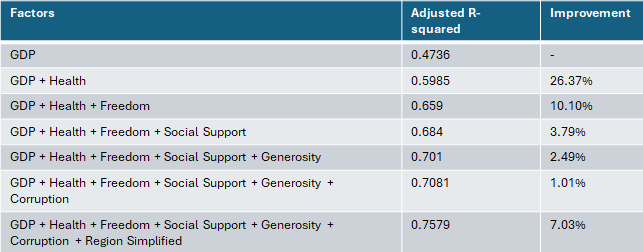
Most Important Factors
An incremental approach has been applied to see- addition of which variable improved the model what percent as below:
Research Question 2: Is there a significant difference in happiness scores between high-income and low-income countries?
Null Hypothesis (𝑯𝟎): There is no significant difference in the mean happiness scores between high-income and low-income countries,
𝐻0: 𝜇_ℎ𝑖𝑔ℎ = 𝜇_𝑙𝑜𝑤
Alternative Hypothesis (𝑯𝟏): There is a significant difference in the mean happiness scores between high-income and low-income countries,
𝐻1: 𝜇_ℎ𝑖𝑔ℎ ≠ 𝜇_𝑙𝑜𝑤
Box plot of mean of happiness score for each income group
# Define high and low-income groups based on GDP
median_gdp <- median(happiness_allVar$GDP, na.rm = TRUE)

# Create IncomeGroup variable: High and Low based on GDP
happiness_inf <- happiness_allVar %>%
  mutate(IncomeGroup = ifelse(GDP > median_gdp, "High", "Low"))

ggplot(happiness_inf, aes(x = IncomeGroup, y = Score, fill = IncomeGroup)) +
  geom_boxplot() +
  labs(title = "Happiness Score by Income Group",
       x = "Income Group", y = "Happiness Score") +
  theme_minimal()
Conditions to Make Inference
- Independence: we assume World Happiness Data collection method ensures independent sampling and the data has been collected randomly
- Sample size: we can investigate the sample size using the following code. According to the income group sizes, the “High” and “Low” groups both have above 30 observations (433 and 435, respectively), meeting the sample size requirement
happiness_inf %>%
group_by(IncomeGroup) %>%
summarise(mean_score = mean(Score, na.rm = TRUE), n = n())| ABCDEFGHIJ0123456789 |
IncomeGroup <chr> | mean_score <dbl> | n <int> | ||
|---|---|---|---|---|
| High | 6.189062 | 433 | ||
| Low | 4.884434 | 435 |
- Normality: The distribution looks nearly normal
#gdp_data <- na.omit(happiness_allVar$GDP)

# Create a data frame for plotting
gdp_df <- data.frame(GDP = happiness_allVar$GDP)

# Plot histogram with overlaid normal distribution curve
ggplot(gdp_df, aes(x = GDP)) +
  geom_histogram(aes(y = ..density..), bins = 30, fill = "skyblue", color = "black") +
  stat_function(fun = dnorm,
                args = list(mean = mean(happiness_allVar$GDP), sd = sd(happiness_allVar$GDP)),
                color = "red", size = 1) +
  labs(title = "Distribution of GDP with Normal Curve",
       x = "GDP",
       y = "Density") +
  theme_minimal()
Calculating Observed Difference and Simulating the Test on Null Distribution
- The observed difference is calculated as follows:
obs_diff <- happiness_inf %>%
  specify(Score ~ IncomeGroup) %>%
  calculate(stat = "diff in means",
            order = c("High", "Low"))

obs_diff| ABCDEFGHIJ0123456789 |
stat <dbl> | ||||
|---|---|---|---|---|
| 1.304629 |
- The null distribution is shown below:
set.seed(1234)
null_dist <- happiness_inf %>%
  specify(Score ~ IncomeGroup) %>%
  hypothesize(null = "independence") %>%
  generate(reps = 1000, type = "permute") %>%
  calculate(stat = "diff in means", order = c("High", "Low"))
ggplot(data = null_dist, aes(x = stat)) +
geom_histogram()
p-value Calculation
- P-value calculation shown below:
p_value <- suppressWarnings(null_dist %>%
  get_p_value(obs_stat = obs_diff, direction = "two_sided"))
p_value| ABCDEFGHIJ0123456789 |
p_value <dbl> | ||||
|---|---|---|---|---|
| 0 |
This strongly suggests that we reject the null hypothesis in favor of the alternative hypothesis, which implies that there is a significant difference in happiness scores between high-income and low-income countries.
Conclusion
This analysis is important because it-
- shows how economic, social, and governance factors impact national well-being. About 71% of the variation in happiness scores is explained by GDP, Social Support, Health, Freedom, Generosity, and Corruption
- confirms a significant disparity in happiness between high-income and low-income countries
The limitations of this analysis-
- correlation does not imply causation. Correlation helps identify relationships (such as GDP vs. Score), but to prove causation- controlled experiments, longitudinal studies, strong theoretical backing, etc. are necessary
- not all factors that affect happiness are included — like culture, religion, or political stability, etc.
- a check for overfitting and underfitting is needed using methods like cross validation
- a time series analysis could better capture changes in happiness over time, especially in response to major events like COVID-19